Permutational Multivariate Analysis of Variance (PERMANOVA)
Abstract
Permutational multivariate analysis of variance (PERMANOVA) is a geometric partitioning of variation across a multivariate data cloud, defined explicitly in the space of a chosen dissimilarity measure, in response to one or more factors in an analysis of variance design. Statistical inferences are made in a distribution-free setting using permutational algorithms. The PERMANOVA framework is readily extended to accommodate random effects, hierarchical models, mixed models, quantitative covariates, repeated measures, unbalanced and/or asymmetrical designs, and, most recently, heterogeneous dispersions among groups. Plots to accompany PERMANOVA models include ordinations of either fitted or residualized distance matrices, including multivariate analogues to main effects and interaction plots, to visualize results.
1 Introduction
PERMANOVA is an acronym for “permutational multivariate analysis of variance”1. It is best described as a geometric partitioning of multivariate variation in the space of a chosen dissimilarity measure according to a given ANOVA design, with p-values obtained using appropriate distribution‐free permutation techniques (see Permutation Based Inference; Linear Models: Permutation Methods). The method is semiparametric, motivated by the desire to perform a classical partitioning, as in ANOVA (hence allowing tests and estimation of sizes of main effects, interaction terms, hierarchical structures, random components in mixed models, etc.), while simultaneously retaining important robust statistical properties of rank-based nonparametric multivariate methods, such as the analysis of similarities (ANOSIM2), namely, (1) the flexibility to base the analysis on a dissimilarity measure of choice (such as Bray–Curtis, Jaccard, etc.) and (2) distribution-free inferences achieved by permutations, with no assumption of multivariate normality. Thus, PERMANOVA opens the door for formal partitioning of multivariate data in response to complex experimental designs in a wide variety of contexts: there may be more response variables than sampling units, data may be severely non-normal, zero‐inflated, ordinal or qualitative (e.g., responses to questionnaires, DNA/RNA sequences, allele frequencies, amino acids, or protein data). Although originally motivated by ecological studies, where variables usually consist of counts of abundances (or percentage cover, frequencies, or biomass) for a large number of species, PERMANOVA is now used across many fields, including chemistry, social sciences, agriculture, medicine, genetics, psychology, economics, and more.
2 Derivation
2.1 The Pseudo F Statistic
Let Y be a matrix of N rows (sampling units) by p columns (variables). Let D = {dij}, i = 1,…, N; j = 1,…, N consist of the distances or dissimilarities between every pair (i, j) of sampling units. The first major milestone in the development of PERMANOVA was the basic achievement of direct partitioning of dissimilarity-based multivariate spaces in response to multiway ANOVA designs3-9. Most similarities S = {sij} can also be reexpressed10 as dissimilarities dij = 1.0 − sij. A direct partitioning of distance matrices having Euclidean metric properties10-12 was extended to semimetric dissimilarities6, 9, having only the properties13 of symmetry (i.e., dij = dji), and that dij ≥ 0 and dii = 0 ∀ i, j.
Consider matrix . Centering the elements of this matrix by row-means, , column-means, , and the overall mean, , gives Gower's matrix G = {gij} = {}. Let X be an (N × g) design matrix whose columns are indicators coding for groups (levels) of an ANOVA factor in a one-way design (e.g., an intercept and orthogonal contrasts7). We can then obtain a projection (hat) matrix H = X[X′X]− 1X′, derived from the normal equations used in linear regression14, 15.
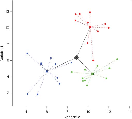
When Euclidean distances are used, then the PERMANOVA sums-of-squares are each equal to the sum of the classical univariate sums of squares across the original variables7, 16; that is, , where is the univariate among-group sum-of-squares for variable k = 1,…, p (and similarly for each of SSR and SST). Hence, pseudo F on Euclidean distances is the same as the F statistic used in classical redundancy analysis (RDA)17, 18. Distance-based redundancy analysis (dbRDA7, 8), equivalent to PERMANOVA, is an RDA on the orthogonal principal coordinates (PCOs) of matrix G based on a chosen (potentially non-Euclidean) dissimilarity measure. However, direct partitioning of matrix G obviates the need for any eigenvector decomposition into PCOs or any corrections for negative eigenvalues that might arise for semimetric (or non-Euclidean-embeddable) dissimilarities8. Furthermore, PERMANOVA on one response variable using Euclidean distance yields the classical univariate F statistic19. So, PERMANOVA can also be used to do univariate ANOVA, but where p values are obtained by permutation20, thus avoiding the assumption of normality.
2.2 Inference
The second major milestone, achieved more-or-less simultaneously, was the development of appropriate permutation algorithms21, 22 for achieving rigorous tests of individual terms in complex ANOVA designs, specifically by conditioning on other terms in the model23, 24 and using expectations of mean squares to identify correct permutable units25, 26. In some cases (e.g., tests of interactions), only asymptotically exact p-values are readily obtainable, for example, via permutation of residuals under a reduced model27, although synchronized permutations28 might be possible.
For cases where there are too few possible permutations to achieve a precise p-value for inferences at a suitably small level of significance, approximate p-values can be obtained using Monte Carlo random draws from the asymptotic permutation distribution29. Specifically, each of the numerator and denominator of pseudo F is asymptotically distributed as a linear form in chi‐square random variables, with coefficients being the eigenvalues from a PCO of matrix G29.
3 Assumptions
3.1 Exchangeability and the Linear Model
PERMANOVA makes no explicit assumptions regarding either the distributions of original variables in Y or the distributions of dissimilarities in D. For a given test, PERMANOVA assumes only exchangeability30, 31 of permutable units under a true null hypothesis. PERMANOVA is only “nonparametric”9 for the one-way case. Inferences remain distribution-free, but PERMANOVA applies a linear model to the dissimilarity space; interactions are defined by reference to additive main effects. Indeed, a key motivation for the development of PERMANOVA was to perform tests for interaction7, 8; PERMANOVA is a classical partitioning in the Euclidean space defined by the full set of PCO axes7, 8. Consequently, the dissimilarity measure will have an important bearing on results, much more so than for rank-based tests, such as ANOSIM2. Hence, in practice, values in matrix D should be neither over-ridden with repeated values at either an upper or lower bound nor dominated by undefined or erratic values, as can occur for sparse data32, 33. Judicious choice of dissimilarity measure32, 34 or pooling of small-scale replicates33 is often well advised.
3.2 Homogeneity of Multivariate Dispersions
Both ANOSIM and the Mantel test are extremely sensitive to differences in dispersions among groups; however, PERMANOVA (like ANOVA) is very robust to heterogeneity for balanced designs but not unbalanced designs35. Furthermore, PERMANOVA, unlike ANOSIM or traditional MANOVA, is not sensitive to differences in correlation structure (shape) among groups35-37.
A test for homogeneity of multivariate dispersions (PERMDISP) in the space of the chosen dissimilarity measure can be done, either to accompany PERMANOVA or in its own right38. This test compares within-group spread among groups using the average value of the distances from individual observations to their own group centroid38-41. The specific directions of distances are not taken into account, so PERMDISP, like PERMANOVA, does not identify differences in the shapes of data clouds among groups, only their relative spread.
4 Extensions
From a PERMANOVA partitioning, direct multivariate dissimilarity-based analogues to familiar univariate statistical constructs in classical ANOVA and regression models are easily identified. This includes partitioning for unbalanced designs (e.g., Type I, Type II, or Type III SS44), pairwise comparisons or a priori contrasts1, inclusion of quantitative covariates1, measurements of precision33, or information criteria for model selection (such as AIC, AICc, or BIC1, 45).
Importantly, PERMANOVA models can include random effects, interaction terms, and hierarchical (nested) structures, with concomitant attendant logical inferences, but in a distribution-free setting. Construction and interpretation of PERMANOVA models rely heavily on the notion of expectations of mean squares (EMS46). For example, classical EMS47-49 are used to correctly construct pseudo F statistics1, identify correct permutable units for a given null hypothesis26, and estimate components of variation46.
Components of variation in PERMANOVA models are calculated using direct analogues to univariate unbiased ANOVA estimators of variance components46 and expressed in units of dissimilarity50. To maintain a distribution-free approach, bootstrapping can be used (each term requiring a specific algorithm within the context of the full multifactor model51) to estimate and compare the sizes of these components52.
All of these constructs boil down to their univariate counterparts for one variable in Euclidean space but, importantly, allow for broad utility when considered for high‐dimensional multivariate systems based on a dissimilarity measure of choice. In ecology, PERMANOVA facilitates the analysis of beta diversity (variation in community structure) across multiple spatial or temporal scales, which is quantified directly by such components of variation53.
5 Plots to Accompany PERMANOVA
Patterns among sampling units can be visualized by a suitable ordination of matrix D, including (i) PCO analysis54; (ii) metric multidimensional scaling (mMDS55, 56); or (iii) nonmetric MDS (nMDS57). Patterns may be readily apparent in such plots for small-to-modest sampling designs, but additional plots described here – specifically, dissimilarity-based analogues to main-effects plots, interaction plots and residual plot – can greatly improve one's understanding of “what PERMANOVA sees” when performing the partitioning and associated tests.
5.1 Distances among Centroids
The number of individual sampling units in complex ANOVA designs may become quite large. Thus, visualizing patterns across factor levels can be difficult; stress (see shepard diagram) in metric or nMDS plots of replicates often exceeds the rule of thumb for interpretability (i.e., stress >0.2). Typically, interest lies in examining the relative positions of group centroids in the space of the dissimilarity measure; this is precisely as in univariate analysis, where plots of means are generally more useful than are plots of raw data. This is achieved by ordination of distances among centroids.
If D contains Euclidean distances, then the distances among centroids are equivalent to Euclidean distances among the arithmetic averages calculated separately for each variable. This equivalence does not hold, however, for non-Euclidean dissimilarities. Distances among centroids based on some other chosen dissimilarity measure are calculated as follows: (i) obtain the full set of PCO axes from matrix G, with each axis having been standardized by the absolute value of its respective eigenvalue; (ii) calculate arithmetic averages for each group separately along each PCO axis; (iii) for every pair of centroids (ℓ, ℓ′), (ℓ = 1,…, g) and (ℓ′ = 1,…, g), calculate Euclidean distances separately in each of the two sets: one based on PCO axes corresponding to non-negative eigenvalues and one based on those corresponding to negative eigenvalues , if any; and (iv) the (g × g) matrix of distances among centroids in the space of the dissimilarity measure is then , where .
Distances among centroids can also be calculated directly from matrix G. For example, consider a one-way ANOVA model with nℓ sampling units in group ℓ and . Let (i ∈ ℓ) denote an indicator for the subset of the i = 1,…, N observations that occur in group ℓ. An “averaged” (g × g) Gower matrix can be obtained as , where . A suitable back-transformation yields the desired distances among every pair of centroids: , obviating the need for PCO axes.
5.2 “Main Effects” Plots, “Interaction” Plots, and “Residual” Plots
In multifactor ANOVA, interest lies in visualizing differences among factor-level centroids as well as the amount of variation attributable to different factors. One may calculate distances among centroids corresponding to the main-effect levels for each factor in turn and place all of these in a single ordination. Such a plot of “main effects,” particularly using metric MDS to preserve the original dissimilarity scale, shows the relative importance of factors, generally reflecting the relative sizes of estimated components of variation from the PERMANOVA partitioning.
Another natural ordination plot of interest is the multivariate direct analogue to an “interaction” plot in the space of the dissimilarity measure. One can do metric or nonmetric MDS (or PCO) on distances among centroids that correspond to individual cells defined by combinations of factor levels (averaging replicates within cells). Such a plot will not only show effects of individual factors but also (potentially) provide insights into the nature of any interactions detected between the factors.
A factor of primary interest may be statistically significant in a PERMANOVA partitioning of the full model, but its effects may be totally obscured by some other dominant factor(s) or covariate(s) in an ordination. Although plots of distances among centroids may shed some light on minor effects, a dissimilarity-based multivariate analogue to a residual plot, from which the variation due to dominant (but perhaps nuisance) factors or covariates has been removed, is desirable.
An (N × N) “residualized” Gower matrix is attainable directly as G[R] = (I − H)G(I − H), where H is the usual “hat” matrix calculated on some model matrix X containing all terms (factors, covariates, etc.) the effects of which one wishes to remove. A “residualized” distance matrix is then obtained as , where . Any of the usual ordination methods (PCO, mMDS, or nMDS) may then be constructed in the usual way from this matrix of residualized distances.
6 Ecological Examples
6.1 Four-Factor Mixed Model: Okura Estuary
Consider a study of potential effects of sedimentation on intertidal soft-sediment fauna in the Okura estuary, near Auckland, New Zealand58. Sites were classified a priori from earlier hydrological studies as having a high, medium, or low probability of sediment deposition. Thus, n = 6 sediment cores (13 cm diameter × 15 cm deep) were sampled randomly from each of the 15 sites, 5 within each of these 3 depositional types of environments. Sampling was repeated a total of six times in 2001–2002: once after a relatively dry period and once 7–10 days after a heavy rainfall event in each of the three seasons: winter, spring, and summer. Abundances of p = 73 taxa were recorded from a total of N = 540 cores in a four-factor design: Season (fixed with three levels: winter, spring, or summer), Rainfall (fixed with two levels: rain or dry), Deposition (fixed with three levels: high, medium, or low), and Site (random with 15 levels, nested within Deposition).
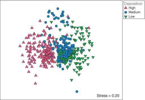
Ordination (nMDS) done directly on the full dissimilarity matrix (Bray–Curtis on fourth-root transformed data) has high stress (∼0.20), and although one may discern a pattern of differences between assemblages from different depositional environments, there is a lot of overlap (Figure 2), and any labeling scheme attempting to show season or rainfall effects is simply uninterpretable, due to high residual variation.
PERMANOVA partitioning shows that spatial effects are the strongest, with Deposition, Site, and the Residual contributing the largest components of variation to the overall model (Table 1). Small-scale spatiotemporal variation, identifiable from statistically significant high-order interactions of temporal factors with Site (Table 1, p < 0.001), was also apparent. Although there was no evidence for a three-way interaction (Season × Rainfall × Deposition; p > 0.48), effects of depositional environments varied across seasons and in different weather conditions (Season × Deposition and Season × Rainfall; p < 0.01).
| Source | df | SS | MS | Pseudo F | p | Component | Var | SD |
|---|---|---|---|---|---|---|---|---|
| Season | 2 | 25 092 | 12 546 | 8.419 | 0.0001 | Fixed | 61.42 | 7.84 |
| Rainfall | 1 | 3965 | 3965 | 2.940 | 0.0138 | Fixed | 9.69 | 3.11 |
| Deposition | 2 | 217 580 | 108 790 | 5.443 | 0.0003 | Fixed | 493.34 | 22.21 |
| Site (Deposition) | 12 | 239 850 | 19 987 | 23.050 | 0.0001 | Random | 531.12 | 23.05 |
| Season × Rainfall | 2 | 11 206 | 5603 | 4.236 | 0.0001 | Fixed | 47.58 | 6.90 |
| Season × Deposition | 4 | 11 126 | 2782 | 1.867 | 0.0051 | Fixed | 21.52 | 4.64 |
| Rainfall × Deposition | 2 | 3400 | 1700 | 1.261 | 0.2574 | Fixed | 3.91 | 1.98 |
| Season × Site(Deposition) | 24 | 35 763 | 1490 | 1.719 | 0.0001 | Random | 51.92 | 7.21 |
| Rainfall × Site(Deposition) | 12 | 16 182 | 1349 | 1.555 | 0.0004 | Random | 26.74 | 5.17 |
| Season × Rainfall × Deposition | 4 | 5232 | 1308 | 0.989 | 0.4807 | Fixed | 0.00 | 0.00 |
| Season × Rainfall × Site(Deposition) | 24 | 31 745 | 1323 | 1.525 | 0.0001 | Random | 75.58 | 8.69 |
| Residual | 450 | 390 200 | 867 | – | – | Random | 867.12 | 29.45 |
| Total | 539 | 991 340 | – | – | – | – | – |
- Pseudo F statistics were calculated for each term using direct analogues to univariate expectations of mean squares (EMS); p-values were obtained using 9999 permutations under a reduced model. Each term is identified as contributing either a fixed or random component to the overall model; “Var” gives the estimated sizes of components of variation, based on multivariate analogues to the classical ANOVA unbiased estimators; “SD” gives the square root of these values, so is in Bray–Curtis units. Nb: Estimates of components of variation (Var) were calculated after pooling (removing) the term “Season × Rainfall × Deposition,” which originally had a negative estimate, so its contribution was set to zero59.
A main-effects plot clearly shows that depositional effects are the strongest, especially contrasting high versus either medium or low depositional areas along mMDS axis 1 (Figure 3a). Seasonal effects are apparent along mMDS axis 2 (from winter to spring to summer), while the contrast of rain versus dry was relatively much smaller (Figure 3a). This mirrors the relative sizes of these main effects in the PERMANOVA partitioning: Deposition, followed by Season, then Rainfall (Table 1). An interaction plot of the 18 Season × Rainfall × Deposition cell centroids not only shows the same pattern but also shows that seasonal effects (along mMDS axis 2) are much larger in high depositional environments (right-hand side of the plot) than for either the medium or low depositional environments. Pairwise comparisons (not shown here) further support these general conclusions.

6.2 Hierarchical Design with a Quantitative Covariate: Kelp Holdfasts
Anderson et al.50 studied organisms colonizing holdfasts of the kelp, Ecklonia radiata; samples were collected according to a spatially structured hierarchical sampling design along the northeast coast of New Zealand. There were four locations (separated by hundreds of kilometers from north to south: Berghan Point, Home Point, Leigh, and Hahei); two sites within each location (separated by hundreds of meters to kilometers); two areas within each site (separated by tens of meters); and n = 5 replicate holdfasts (separated by meters) within each area. A total of 351 taxa from 15 different phyla were enumerated/quantified from these N = 80 holdfasts.
Interest lies in quantifying multivariate variation in assemblage structure at each spatial scale (beta diversity34, 53) while taking into account natural variation in the sizes of holdfasts; the volume of each holdfast was measured using water displacement. Bray–Curtis dissimilarities were calculated on fourth-root transformed values.
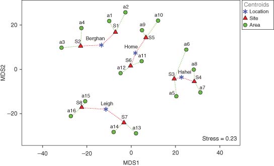
PERMANOVA partitioning using a sequential (Type I) sum of squares showed the greatest component of variation was the residual (smallest scale), followed by locations, areas, and then sites; the latter two scales were comparable in their effect sizes (Table 2). Volume, although statistically significant (p < 0.001), was less important than any of the spatial factors. For this example, stress is relatively high even for a “main-effects” plot of distances among centroids (Figure 4), reflecting the high dimensionality of this multivariate system. Nevertheless, the distinctiveness of the four locations is quite apparent, the centroids for sites within them appear like satellites around each one, while area-level centroids appear, in turn, as satellites around each site centroid (Figure 4). Similar patterns were shown in a nMDS plot (stress = 0.12) and in a three-dimensional mMDS plot (stress = 0.13) of these distances (not shown). The “balance” of the two satellites (i.e., being opposite and equidistant) around any particular centroid in this fully nested design was seen more perfectly in the 3D mMDS plot.
| Source | df | SS | MS | Pseudo F | p | Component | Var | SD |
|---|---|---|---|---|---|---|---|---|
| Volume | 1 | 8720 | 8720 | 2.467 | 0.0003 | Fixed | 64.81 | 8.05 |
| Location | 3 | 23 256 | 7752 | 3.289 | 0.0001 | Random | 304.47 | 17.45 |
| Site (Location) | 4 | 10 139 | 2535 | 1.798 | 0.0002 | Random | 113.28 | 10.64 |
| Area (Site(Location)) | 8 | 11 286 | 1411 | 1.750 | 0.0001 | Random | 121.63 | 11.03 |
| Residual | 63 | 50 778 | 806 | – | – | Random | 806.00 | 28.39 |
| Total | 79 | 104 180 | – | – | – | – | – |
- The analysis was based on Bray–Curtis dissimilarities of fourth-root transformed values and pseudo F statistics were calculated for each term using direct analogues to univariate expectations of mean squares (EMS); p-values were obtained using 9999 permutations under a reduced model. Each term is identified as contributing either a fixed or random component to the overall model; “Var” gives the estimated sizes of components of variation, based on multivariate analogues to the classical ANOVA unbiased estimators; “SD” gives the square root of these values, so is in Bray–Curtis units. Nb: Interactions of each of the ANOVA factors (Location, Site, or Area) with Volume were omitted from the model, as the p-values for all of these interaction terms were >0.23.
6.3 Randomized Block Design: Plankton
A study by Winsor and Clarke60, 61 investigated the catch of several types of plankton using two nets hauled horizontally, one being 2 m below the other. Ten hauls were made with the pair of nets at depth positions of 29 and 31 m, respectively. Data were transformed to logarithms of the catch numbers for each of p = 5 plankton types.
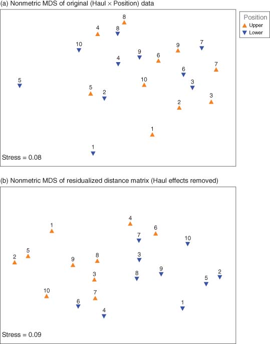
This yielded a randomized block design. Ordination of individual sampling units showed no strong effect of position on these plankton assemblages – the two different symbols are quite well mixed (Figure 5a). However, PERMANOVA clearly detected a significant effect of “Position” (Table 3a). The key is PERMANOVA's ability to partition, hence partial out, the (random) effects due to different hauls (equivalently, to identify the “paired” nature of the nets in this design), thereby diminishing the residual and yielding greater power for the factor of interest: the position of the nets (upper vs lower). A useful plot here is the nMDS plot of residualized distances, having removed the (dominating) effects of hauls, in which the contrast (separation) between plankton assemblages in upper versus lower nets is now quite obvious (Figure 5b). Not surprisingly (given Figure 5a), no statistically significant effects of “position” would be detected if variation among hauls were to be ignored (Table 3b).
| Source | df | SS | MS | Pseudo F | p | Component | Var | SD |
|---|---|---|---|---|---|---|---|---|
| (a) Including Hauls | ||||||||
| Haul | 9 | 434.59 | 48.29 | 6.605 | 0.0001 | Random | 20.49 | 4.53 |
| Position | 1 | 43.11 | 43.11 | 5.897 | 0.0270 | Fixed | 3.58 | 1.89 |
| Residual | 9 | 65.79 | 7.31 | – | – | Random | 7.31 | 2.70 |
| Total | 19 | 543.49 | – | – | – | – | – | |
| (b) Ignoring Hauls | ||||||||
| Position | 1 | 43.11 | 43.11 | 1.551 | 0.2167 | Fixed | 1.53 | 1.24 |
| Residual | 18 | 500.38 | 27.80 | – | – | Random | 27.80 | 5.27 |
| Total | 19 | 543.49 | – | – | – | – | – | |
- First, an analysis is done (a) that takes into account the variation among hauls (as in a randomized block design); a second (erroneous) analysis (b) is done as a simple one-way design, treating the hauls merely as replicates, so ignoring the pairing of the nets. Pseudo F statistics were calculated for each term using direct analogues to univariate expectations of mean squares (EMS); p-values were obtained using 9999 permutations under a reduced model for analysis (a) and 9999 raw data permutations for analysis (b). Each term is identified as contributing either a fixed or random component to the overall model; “Var” gives the estimated sizes of components of variation, based on multivariate analogues to the classical ANOVA unbiased estimators and “SD” gives the square root of these values, so is in Bray–Curtis units.
7 Conclusions
PERMANOVA provides a useful statistical tool for the analysis of multivariate data on the basis of Euclidean distances or non-Euclidean-embeddable dissimilarity measures. Its utility, in many ways, simply mirrors that of classical ANOVA62, yet, as a geometric partitioning, it extends to something much broader and even more widely applicable, allowing rigorous meaningful analysis of high-dimensional systems, even those having variables with extremely non-normal or overdispersed behavior. It is not restricted by distributional assumptions and has recently been extended also to accommodate heterogeneity of within-group dispersions.
Acknowledgments
This work was supported by a James Cook Fellowship from the Royal Society of New Zealand. PERMANOVA would not exist were it not for B. H. McArdle, P. Legendre, K. R. Clarke, C. J. F. ter Braak, J. Robinson, and A. J. Underwood. I especially thank R. N. Gorley, without whom many of the most useful and elegant extensions to PERMANOVA and associated ordinations could not have been so readily achieved.
Related Articles
Multiresponse Permutation Procedures; Permutation Tests: Multivariate; Similarity, Dissimilarity, and Distance, Measures of; Multivariate Analysis of Variance (MANOVA); Redundancy Analysis; Multivariate


